Table of Contents
- Introduction
- Installing and Importing
- Table of Contents
- Creating Data Frames
- Previewing Data
- Sorting
- Selecting/Querying
- Modifying Data Frames
- Dates and Time
- Plotting
Introduction
This article overviews how to quickly set up and get started with the pandas data analysis library. It also lists common code snippets for parsing, loading, and transforming data. For more detailed documentation on pandas’ more advanced features (e.g. plot styling and combining data frames) you’ll need to refer to other sources.
Installing and Importing
First we need to install python and the pip package manager. If you don’t already have them, you can use pyenv to easily install them (tested on Ubuntu and OS X). On Ubuntu, you can follow these instructions to get pyenv. On OS X you can just use brew:
1
brew install pyenv
Once you have pyenv, you can install and configure the desired python version as follows:
1
2
3
4
# Install the desired python version - e.g. 3.4.3
pyenv install 3.4.3
# Set it up as a global version - pyenv will reconfigure your PATH accordingly
pyenv global 3.4.3
Now we can use pip to install pandas, the ipython shell, and jupyter.
1
pip install pandas ipython[all] jupyter
The last two libraries will allow us to create web base notebooks in which we can play with python and pandas. If you don’t know what jupyter notebooks are you can see this tutorial.
Next, we need to start jupyter. I find it useful to store all notebooks on a cloud storage or a folder under version control, so I can share between multiple machines. This can be achieved with an additional parameter as follows:
1
jupyter notebook --notebook-dir=~/Dropbox/notebooks
Next, we need to import pandas in the first cell of the jupyter notebook.:
1
import pandas
Table Of Contents
When we have a long notebook, it is useful to have an automatically generated table of contents (TOC). The following code (Borrowed from this post on StackOverflow) installs the TOC jupyter plugin, i.e.:
1
2
3
4
5
6
7
8
9
10
## download
mkdir toc
cd toc
wget https://raw.githubusercontent.com/minrk/ipython_extensions/master/nbextensions/toc.js
wget https://raw.githubusercontent.com/minrk/ipython_extensions/master/nbextensions/toc.css

## install and enable
cd ..
jupyter-nbextension install --user toc
jupyter-nbextension enable toc/toc
Then we need to restart the kernel and make the first cell “Markdown” type and add the following:
1
2
**Table of Contents**
<div id="toc"></div>
When you save the TOC should appear.
Creating Data Frames
Data frames are the central concept in pandas. In essence, a data frame is table with labeled rows and columns. Data frames can be created from multiple sources - e.g. CSV files, excel files, and JSON.
Loading CSV files
Loading a CSV file as a data frame is pretty easy:
1
data_frame = pandas.read_csv('file.csv', sep=';')
Sometimes the CSV file contains padding spaces in front of the values. To ignore them use the skipinitialspaces parameter:
1
pandas.read_csv('file.csv', sep=';', skipinitialspace=True)
If the padding white spaces occur on both sides of the cell values we need to use a regular expression separator. In this case, we need to use the ‘python’ processing engine, instead of the underlying native one, in order to avoid warnings. This will degrade the performance a bit:
1
pandas.read_csv('file.csv', sep='\s*;\s*', skipinitialspace=True, engine='python')
Sometimes we need to sample the data before loading it, as it is too big to fit in memory. This can be achieved following this approach.
Hardcoded Dataframes
Hardcoded data frames can be constructed by providing a hash of columns and their values.
1
2
3
4
5
6
7
import numpy as np

df = pandas.DataFrame({
   'col1': ['Item0', 'Item0', 'Item1', 'Item1'],
   'col2': ['Gold', 'Bronze', 'Gold', 'Silver'],
   'col3': [1, 2, np.nan, 4]
})
We will reuse this data frame in some subsequent examples.
Previewing Data
To preview the data and the metadata of a dataframe you can use the following functions:
1
2
3
4
5
6
7
8
9
10
11
12
13
14
15
16
17
18
19
20
21
22
23
# Displays the top 5 rows. Accepts an optional int parameter - num. of rows to show
df.head()

# Similar to head, but displays the last rows
df.tail()

# The dimensions of the dataframe as a (rows, cols) tuple
df.shape

# The number of columns. Equal to df.shape[0]
len(df)

# An array of the column names
df.columns

# Columns and their types
df.dtypes

# Converts the frame to a two-dimensional table
df.values

# Displays descriptive stats for all columns
df.describe()
Sorting
The sort_index method is used to sort the frame by one of its axis indices. The axis is either 0 or 1 - row/column axis respectively:
1
2
# Sort rows descendingly by the index
df.sort_index(axis=0, ascending=False)
We can also sort by one or multiple columns:
1
df.sort_values(by=['col2', 'col1'], ascending=False)
Selecting/Querying
Individual columns can be selected with the [] operator or directly as attributes:
1
2
3
4
5
6
7
8
# Selects only the column named 'col1';
df.col1

# Same as previous
df['col1']

# Select two columns
df[['col1', 'col2']]
You can also select by absolute coordinates/position in the frame. Indices are zero based:
1
2
3
4
5
6
7
8
# Selects second row
df.iloc[1]
# Selects rows 1-to-3
df.iloc[1:3]
# First row, first column
df.iloc[0,0]
# First 4 rows and first 2 columns
df.iloc[0:4, 0:2]
Most often, we need to select by a condition on the cell values. To do so, we provide a boolean array denoting which rows will be selected. The trick is that pandas predefines many boolean operators for its data frames and series. For example the following expression produces a boolean array:
1
2
# Produces and array, not a single value!
df.col3 > 0
This allows us to write queries like these:
1
2
3
4
5
6
7
8
9
10
11
12
13
14
# Query by a single column value
df[df.col3 > 0]

# Query by a single column, if it is in a list of predefined values
df[df['col2'].isin(['Gold', 'Silver'])]

# A conjunction query using two columns
df[(df['col3'] > 0) & (df['col2'] == 'Silver')]

# A disjunction query using two columns
df[(df['col3'] > 0) | (df['col2'] == 'Silver')]

# A query checking the textual content of the cells
df[df.col2.str.contains('ilver')]
Modifying Data Frames
Pandas’ operations tend to produce new data frames instead of modifying the provided ones. Many operations have the optional boolean inplace parameter which we can use to force pandas to apply the changes to subject data frame.
It is also possible to directly assign manipulate the values in cells, columns, and selections as follows:
1
2
3
4
5
6
7
8
9
10
11
12
13
14
15
16
17
18
# Modifies the cell identified by its row index and column name
df.at[1, 'col2'] = 'Bronze and Gold'

# Modifies the cell identified by its absolute row and column indices
df.iat[1,1] = 'Bronze again'

# Replaces the column with the array. It could be a numpy array or a simple list.
#Could also be used to create new columns
df.loc[:,'col3'] = ['Unknown'] * len(df)

# Equivalent to the previous
df.col3 = ['Unknown'] * len(df)

# Removes all rows with any missing values.
df.dropna(how='any')

# Removes all rows with all missing values.
df.dropna(how='all')
It is often useful to create new columns based on existing ones by using a function. The new columns are often called Derived Characteristics:
1
2
3
4
5
6
7
8
9
10
11
def f(x):
    return x + ' New Column';

# Uses the unary function f to create a new column based on an existing one
df.col4 = f(df.col3)

def g(x, y):
    return x + '_' + y

# Uses the 2-arg function g to create a new column based on 2 existing columns
df.col4 = g(df.col3, df.col2)
Dates and Time
When loading data from a CSV, we can tell pandas to look for and parse dates. The parse_dates parameters can be used for that. In the most typical case, you would pass a list of column names as parse_dates:
1
dates_df = pandas.read_csv('test.csv', sep=';', parse_dates=['col1', 'col2'])
This will work for most typical date formats. If it does not (i.e. we have a non-standard date format) we need to supply our own date parser:
1
2
3
4
5
def custom_parser(s):
    # Specify the non-standard format you need
    return pandas.datetime.strptime(s, '%d%b%Y')

dates_df = pandas.read_csv('test.csv', sep=';', parse_dates=['col1'], date_parser=custom_parser)
Alternatively, if we’ve already loaded the data frame we can change a column from string to a date:
1
dates_df['col2'] = pandas.to_datetime(dates_df['col2'], format='%d.%m.%Y')
For more on date-time formats look at the documentation.
Often we need to work with Unix/Posix timestamps. Converting numeric timestamps to pandas timestamps is easy with the unit parameter:
1
2
# Unit specifies if the time is in seconds('s'), millis ('ms'), nanos('ns') etc.
dates_df['col'] = pandas.to_datetime(dates_df['col'], unit='ms')
If we need to parse Posix timestamps while reading CSVs, we can once again resort to converter functions. In the converter function we can use the pandas.to_datetime utility which accepts a unit parameter:
1
2
3
4
5
def timestamp_parser(n):
    # Specify the unit you need
    return pandas.to_datetime(float(n), unit='ms')

dates_df = pandas.read_csv('test.csv', sep=';', parse_dates=['col1'], date_parser=timestamp_parser)
We can also convert time/timestamp data to Unix epoch numbers:
1
2
# Creates a new numeric column with the timestamp epoch in nanos
dates_df.col4 = pandas.to_numeric(dates_df.col3)
Plotting
Set Up
Pandas uses matplotlib to render graphs, so you need to install it:
1
pip install matplotlib
Before we continue we need to test if matplotlib was set up properly. Open a terminal, start the python interpreter, and type:
1
import matplotlib
If the import works without problems you’re good to go. However, sometimes in OS X you may get the following error:
“RuntimeError: Python is not installed as a framework. The Mac OS X backend will not be able to function correctly if Python is not installed as a framework. See the Python documentation for more information on installing Python as a framework on Mac OS X. Please either reinstall Python as a framework, or try one of the other backends. If you are Working with Matplotlib in a virtual enviroment, see ‘Working with Matplotlib in Virtual environments’ in the Matplotlib FAQ”
If that error occurs, you need to execute the following from terminal:
1
echo "backend: TkAgg" >> ~/.matplotlib/matplotlibrc
This will set the proper matplotlib backend, as discussed here.
Now we can import the matplot library in one of the jupyter notebook cells:
1
import matplotlib.pyplot as plt
There is one last configuration to complete before we can display plots in the web notebook. We need to tell jupyter to display the matplotlib plots as images in the notebook itself. To do so, type the following command in one of the notbook cells:
1
2
# Will allow us to embed images in the notebook
%matplotlib inline
Basic Plotting
In the rest of this section we’ll use the following data frame:
1
2
3
4
5
plot_df = pandas.DataFrame({
    'col1': [1, 3, 2, 4],
    'col2': [3, 6, 5, 1],
    'col3': [4, 7, 6, 2],
})
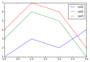
Data frames have a method called plot. By default, it plots a line chart with al numerical columns. The x-axis is the row index of the data frame. In other words, you’re plotting :
1
plot_df.plot()
We can also specify a column for the x-axis:
1
plot_df.plot(x='col1')
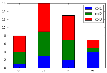
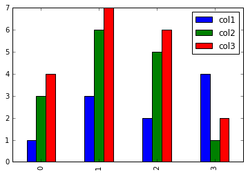
The plot has an optional parameter kind which can be used to plot the data in different type of visualisation - e.g. bar harts, pie chart, or histograms.
Using kind=’bar’ produces multiple plots - one for each row. In each plot, there’s a bar for each cell.
1
2
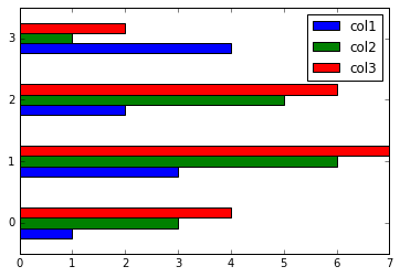
# Use kind='hbar' for horizontal bars, and stacked=True to stack the groups
plot_df.plot(kind='bar')
Boxplots are displayed with the kind=’box’ options. Each box represents a numeric column.
1
plot_df.plot(kind='box')