Parallel Mapping and Reduction

A great deal of programming is about working with collections - e.g. filtering, mapping, reducing lists/sets/dictionaries. If we could parallelise these operations in a way which is transparent to the end programmer, then seemingly serial programs could reap the benefits of parallel hardware behind the scenes.

As we saw in the previous section, applying parallel algorithms often requires access to arbitrary values from the collection - e.g. the middle element. Scala’s List doesn’t lend itself to parallelisation as it is just a pair of a head and a tail. We’ll focus on arrays and trees instead.

Mapping an array in parallel is quite trivial. We just need to divide it in two, and run parallel recursive calls for the two parts. Once the array length reaches a certain threshold, we can use serial mapping.

Similarly, trees can be mapped in parallel by traversing them and running parallel recursive calls for each child. Once we’ve reached a certain threshold depth in the tree, we can start running serial mapping.

Folding/reducing a data structure is more difficult than mapping because, in the general case, computations depend on each other. Let’s assume we have an array val a = Array(3,2,1) and we invoke a.reduceLeft(_ - _). This can not be run in parallel, as the evaluation of (3-2)-1 depends on the evaluation of 3-2.

However, if the reducing function is associative we can run the computations in parallel. A function f is associative iff f(a,f(b,c)) = f(f(a,b),c) for every a, b, and c.

For example def f(a:Int, b: Int) = a+b is associative, because (a+b)+c = a+(b+c). However, def g(a:Int, b: Int) = a-b is not.

Associativity allows us to run things in parallel, because we can “put the brackets” any way we want. More formally, if f is associative then the following expressions are equivalent:

1
2
3
4
5
6
7
8
// Reduce/fold definition
f(a1, f(a2, ... f(an-1, an) ))

// Equivalent if f is associative
val m = n / 2
val firstHalf = f(a1, ... f(am-1, am))
val secondHalf = f(a1, ... f(am+1, an))
f(firstHalf, secondHalf)

In other words, if f is associative we can split the array in parts, compute the reduction of the parts, and then combine/reduce these values with f. These independent sub-reductions can be run in parallel analogously to what we did for map.

Associativity

As we just saw, associativity allows us to reorder a sequence of computations and run them in parallel. Another important property of two-arguement functions is commutativity. A function f is commutative if f(a,b)=f(b,a) for every a and b.

Here are some examples of functions which are both associative and commutative:

• Sum of integers, because (a+b)+c = a+(b+c) and a+b = b+a;
• Multiplication of integers (analogous to summation);
• Union of sets, because \( (A \cup B) \cup C \) = \( A \cup (B \cup C) \) and \( A \cup B \) = \( B \cup A \);
• Intersection of sets (analogous to union);
• Boolean conjunction: (a && b) && c = a && (b && c) and a && b = b && a;
• Boolean disjunction (analogous to conjunction);

Examples of associative but not commutative:

• List concatenation: (a++b)++c = a++(b++c) but a++b = b++a is not always true;
• Matrix multiplication: \( (A \times B) \times C = A \times (B \times C) \) but \( A \times B \) = \( B \times A \) is not always true.

Examples of commutative but not associative:

• Sum of floats: a+b = b+a but (a+b)+c = a+(b+c) may not be true due to the different accumulated roundings.
• Multiplication of floats (analogous to summation);

Week 3: Data Parallelism

There are two main “styles” of parallelism - task and data parallelism. In the task based approach, we distribute the execution of different computations across multiple processing units. Data parallelism is when we run the same computation with different parameters/data on multiple units.

The efficiency of the task parallel approach grows with the number of independent tasks you can break the problem in. On the contrary, data paralelism’s efficiency grows with the quantity of the data.

An example of task parallelism is a client-server system, which has separate threads for serving requests, making requests, etc. An example of data parallelism is a parallel for loop, where an array is subdivided into parts and the body of the loop is run in parallel over all parts.

Data Parallelism in Scala Collections

In Scala, the standard library consists of standard/serial collections and parallel collections. For most collections, there is a parallel alternative prefixed with “Par” - e.g. Set and ParSet. To allow the development of code which works with both serial and parallel collections, there are generic alternatives of all collections which are supertypes of both the serial and parallel versions:

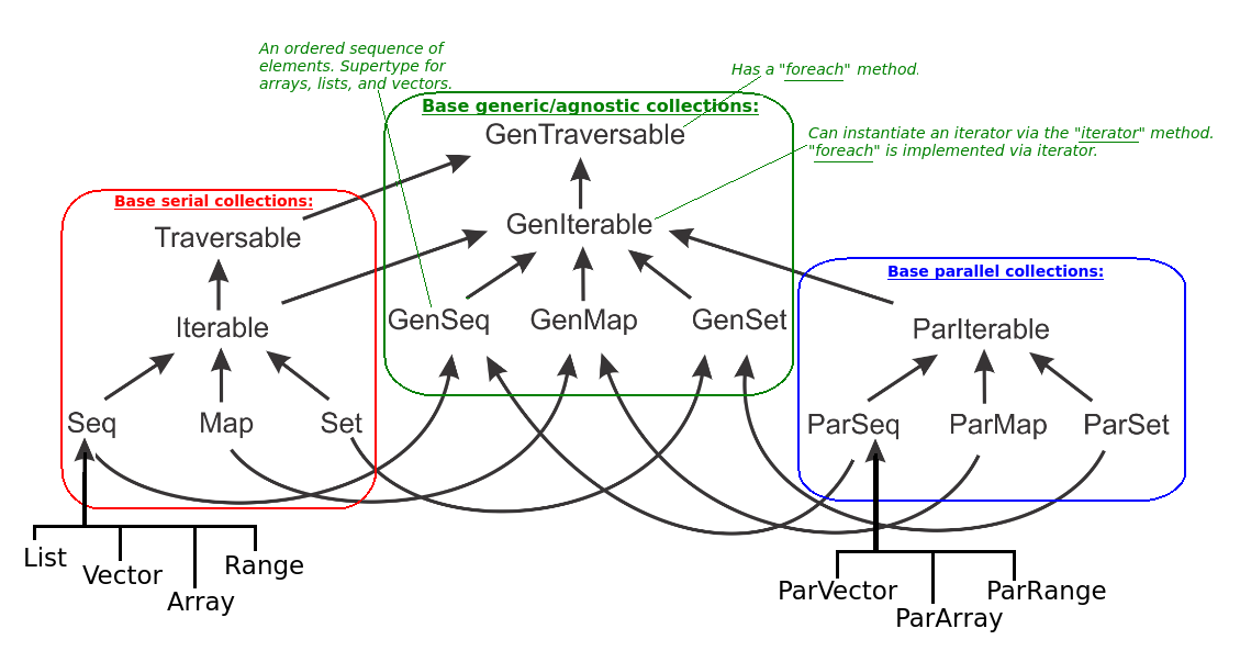
Note that there’s no collection ParList. As discussed List, which is pair of a head element and tail, is not suitable for most parallel operations.

Every collection can be converted to its parallel alternative via the par method. For example:

1
2
3
4
5
6
7
Set(1,2,3).par    // Returns a ParSet instance

Array(1,2,3).par  // Returns a ParArray instance

(1 to 5).par      // Returns a ParRange instance

List(1,2,3).par   // Returns a ParVector instance

Splitters and Combiners

Scala standard collections provide the Iterator interface/trait, which is typical for imperative languages. A simplified version is:

1
2
3
4
trait Iterator[A] {
  def next(): A
  def hasNext: Boolean
}

We can define the sequential fold/reduce operations for every collection that we can convert to an iterator. However, for the parallel reduction we’ll need a way to split the collection in parts which we can process in parallel. Hence, some collections provide Splitters. The simplified trait can be defined as:

1
2
3
4
trait Splitter[A] extends Iterator[A] {
  def split: Seq[Splitter[A]]
  def remaining: Int
}

The split method returns disjoint sub-collections of the present collection. It should be an efficient method with not more than \( O(log(n)) \) complexity. The remaining method returns an estimation of the number of elements in the splitter. Usually, algorithm compare the remaining value to a threshold to determine whether to continue splitting and run the sub-collections in parallel rather than just run sequentially.

Scala standard collections also provide the Builder interface/trait, whose simplified version is:

1
2
3
4
trait Builder[A,Repr] {
  def +=(elem: A): Builder[A,Repr]
  def result: Repr
}

Where Repr is type of a collection - e.g. List, Vector, etc. The += operation adds to the builder. The result method returns the created resulting collection of type Repr.

Having Builder implementations for every collection allows us to implement the serial version of filter in a collection agnostic way:

1
2
3
4
5
6
7
def filter(p: T => Boolean): Repr = {
  val b = newBuilder
  for (x <- this)
    if(p(x))
      b +=x
  b.result
}

In order to implement parallel filter/reduce, we can use appropriate Splitter instances to divide the collection into subparts that can be processed in parallel. Then, we need a way to combine the results of the independent parallel computations in parallel. For this, there’s the Combiner interface:

1
2
3
trait Combiner[A, Repr] extends Builder[A, Repr] {
  def combine(that: Combiner[A, Repr]) :Combiner[A, Repr]
}  

The combine function aggregates the two combiners. It should be faster than \( O(log(n)) \).

The parallel collections in Scala all have splitters and combiners through which the parallel algorithms are implemented in an uniform way.

Week 4: Data Structures for Parallel Computing

We saw that the Combiner interface is a useful tool to implementing parallel data structures in a unified way. But how should we implement efficient combiners for the most commonly used collections?

A combiner for sequences would implement the concatenation operation, while a combiner for sets/maps would implement union. However, arrays can’t be concatenated efficiently and most sets/maps take linear time for union.

Two-Phase Construction

To overcome these problems, most combiners use intermediate data structures. In other words, such combiners work in two phases. Firstly, they efficiently aggregate/combine elements (i.e. using += and combine) into the intermediate data structure. Secondly, they efficiently convert from this intermediate representation to target one (i.e. the Repr type parameter).

For example, the combiner for arrays is implemented with an array list (i.e. ArrayBuffer) of array lists of the actual elements - i.e. ArrayBuffer[ArrayBuffer[T]]. When a new element is added (with +=) to the combiner, it appends it to the last list, which has \( O(1) \) complexity. When two array combiners are concatenated (with combine) their lists of lists are concatenated. This operation is linear with respect to the “outer lists”, but is on average logarithmic with respect to the total number of elements in the two collections. Finally, the underlying array lists can be combined into an array in linear time. This could be further improved by running the concatenation in parallel on multiple processors.

Similarly, we can implement efficient combiners for hash sets and maps. We can partition the hash codes into buckets corresponding to integer ranges. This allows for the element addition and union can be implemented efficiently. Converting back to original collection takes linear time and is parallelisable.

Conc-Trees

We saw that we can implement efficient combiners for arrays, hash sets, and hash maps. But how about trees? If a tree is no balanced then running parallel operations on it can be challenging.

Conc-Trees are binary tree data structures with efficient addition and union operations that maintain its balanced form. It can be used to implement efficient combiners for arrays.