
Table of Contents
- Introduction
- Why Spark (and Scala)
- From Data-Parallel to Distributed Data-Parallel
- Apache Spark vs Hadoop
- Resilient Distributed Dataset (RDD)
- Cluster Topology
- Reduction Operations
- Pair RDDs
- Joins (More Pair RDDs)
- Shuffling and why reduceByKey is good
- Partitioning
- Wide vs Narrow Dependencies
- Structure and Optimisation
- Spark SQL
- More about DataFrames
- Datasets
Introduction
Apache Spark has emerged as the premium tool for big data analysis and Scala is the preferred language for writing Spark applications. I recently took the Big Data Analysis with Scala and Spark course on Coursera and I highly recommend it. It’s a great, intuitive, and accessible introduction to Spark building upon a good understanding of Scala’s standard collections. This post is a summary of the course.
For many constructs, Spark relies heavily on the right implicit definitions and set-up being present. The following snippets are for illustrative purposes only and may not even compile unless you have a properly set-up environment. Consult the Spark documentation and the course lecture notes for exact set up instructions.
Why Spark (and Scala)
R and MATLAB are useful for small data sets - megabytes to gigabytes. They do not scale well when you have huge volumes of data. Spark is a framework that allow us to distribute big data processing on a cluster of machines. In contrast to Hadoop, Spark is much more expressive, interactive, and does not confine us to the map-reduce paradigm. Scala’s functional style is a good match for Spark’s primitives. In fact, Scala’s standard collections match Spark’s nearly 1-to-1.
From Data-Parallel to Distributed Data-Parallel
Data-parallelism is about separating a data structure (e.g. Vector or Matrix) into chunks which can be processed on multiple CPUs or cores. Afterwards, the results of the independent computations are combined to get the final result. Data-parallel operations can be implemented as methods on the aforementioned data structures.
Scala’s standard collection offers many data-parallel data structures. An example of data-parallel enabled collection is a ParSet.
1
2
3
// ParSet.reduce will divide the set into chunks, perform
// the computations in parallel and assemble the result
println(ParSet(1,2,3,4,5).map(_ + 1).reduce( _ + _))
Distributed data parallelism is very similar. The only difference is that instead of CPUs/cores we use separate networked nodes/computers. This introduces concerns like network latency and failure, which we’ll need to account for in all computations.
While Scala’s standard collections are in-memory only, a Spark
Resilient Distributed Dataset (RDD) represents a distributed data
structure whose individual chunks reside on individual machines.
An RDD has very similar methods to Scala’s parallel collections, so we can
still use the beloved map, flatMap, reduce, filter and more.
Thus, the coding patterns are similar as well:
1
2
3
4
5
6
7
// A Spark RDD representing a huge number of integers on multiple nodes.
// It's created via Spark's utility methods.
val numbers: RDD[Int] = ...

// Reduce - under the hood Spark will distribute the computation on multiple
// machines and combine the result.
println(numbers.reduce(_ + _))
Apache Spark vs Hadoop
Hadoop applications consists of a number of map and reduce jobs, which respectively transform the data chunks and combine the intermediate results. To handle job failures, Hadoop persists the output of every job to at least 3 nodes in the cluster, which causes a huge amount of disk and network data transfer.
Spark, on the other hand, loads the persistent data in memory and transforms it on the fly, without persisting the intermediate results back to disk. To achieve this, Spark ensures that RDDs are immutable. Every RDD operation generates a new RDD. If a node crashes, the same sequence of computations can be repeated on the initial RDD to restore the lost information. This makes it unnecessary to store intermediate results to disk and makes Spark much faster than Hadoop in the average case.
Resilient Distributed Dataset (RDD)
Spark is installed on a cluster of nodes/computers.
Whenever we’re running a Spark program, we can get a handle on a utility
instance of a class SparkContext (SparkSession in later versions)
which allows us to instantiate RDDs.
1
2
3
4
5
6
7
8
// Create a config for local Spark execution (single machine)
// and instantiate a SparkContext
val conf: SparkConf = new SparkConf().setMaster("local").setAppName("StackOverflow")
val sc: SparkContext = new SparkContext(conf)

// Use the context to create some RDDs
val intRdd: RDD[Int] = sc.parallelize(List(1,2,3));
val txtRdd: RDD[String] = sc.textFile('hdfs://myFile.txt')
There are two main types of RDD operations - Transformations and Actions.
Transformations take an RDD as input and produce another RDD as output.
Example of transformations are map, filter, flatMap, union, and intersection:
Actions, on the other hand, take an RDD as input and produce a single output
which is not a RDD.
Example of actions are reduce, fold, foreach, sum, and saveAsTextFile.
Transformations are lazy, while actions are evaluated eagerly:
1
2
3
4
5
6
7
8
9
10
val intRdd: RDD[Int] = sc.parallelize((1 to 1000).toList);

// The following will not be evaluated immediately.
// "transformed" is a lazily evaluated collection
val transformed = intRdd.map(_ * 2);

// Reduce is an action and is computed eagerly.
// It will force the lazy computation embedded in "transformed" to run
// and then will sum all the number.
val result = transformed.reduce(_ + _)
Transformation laziness is a good performance improvement. Whenever an action forces an actual computation, Spark already has a number of accumulated transformations, which it can reshuffle and combine for faster execution.
However, there is also a downside to laziness. If an RDD is produced by a
transformation from another RDD, and is then used by 2 actions, the transformation
will be performed twice. Thus, RDDs have methods cache and persist, which
preserve the result of the first lazy evaluation in memory or on disk respectively:
1
2
3
4
5
6
7
8
9
10
11
12
val intRdd: RDD[Int] = sc.parallelize((1 to 1000).toList);

// The following will not be evaluate immediately.
// "transformed" will be evaluated  lazily and saved in memory (cache)
val transformed = intRdd.map(_ * 2).cache();

// This will force the lazy computation embedded in "transformed" to run
// and then will sum all the number.
val rddSum = transformed.reduce(_ + _);

// The cached value of "transformed" will be used - it will not run again.
val rddCount = transformed.count();
persist can be customised to save the data on disk, in memory, or on both.
The cache method is in fact a shorthand for persist in memory.
Cluster Topology
A Spark cluster is deployed in a master-worker style topology depicted below.
The master is also called Driver, and executes the user provided commands.
It is the “main method” or the REPL. It provides the SparkContext/SparkSession
instances, via which we can instantiate and process RDDs.
Behind the scenes, the driver schedules the RDD operations on the workers via the
Cluster Manager.
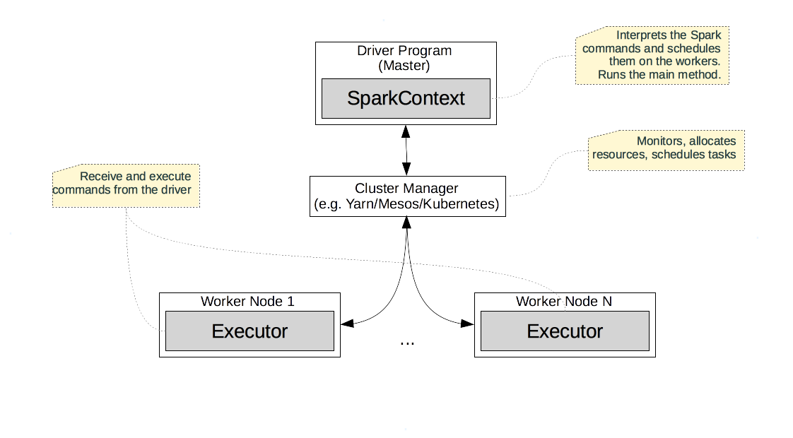
The Cluster Manager controls the resources of the cluster, monitors the nodes, and schedules the individual tasks. The cluster managers are generic and are not Spark specific. Spark is usually used with YARN, Mesos, or Kubernetes.
The Spark workers run processes called executors, which perform computations, read and store persistent data, and provide in-memory caches for RDDs.
Given this topology, a typical Spark script follows these steps. Spark starts on the driver, and allocates the SparkContext/SparkSession instance needed for the application. Then, Spark uses the cluster manager to allocate and connect to a few executors. Afterwards, the driver transfers the application code to the executors. After this setup is complete, the application can finally start. The driver breaks up the application into individual RDD operations and schedules them as tasks on the executors.
In general, transformations (i.e. lazy operations) are accumulated on the master. Actions (eager operations) and the accumulated transformations they depend on are run on the executors. The results of an action (if not persisted) are sent back to the driver, which can use it in the subsequent application control flow.
Reduction Operations
Transformations (e.g. map and filter) are very easy to distribute.
Every node can apply the transformations locally without
transferring data across nodes. However actions like reduce, aggregate,
and fold need to coordinate data exchange across nodes.
In Scala collections, operations like foldLeft, and foldRigth are not parallelizable
and distributable, because the order is important.
As a consequence, Spark RDDs do not support foldLeft, and foldRigth.
However, aggregate, fold, and reduce are parallelisable if the operation is associative.
We can split the collection (e.g. Map, Set, RDD) into parts, operate on them in parallel
and combine the results. This form of computation is called reduce tree,
where a data structure is recursively subdivided, operated on, and the results
are combined.
The fold and reduce methods have a serious limitation. They can only combine
the values of a collection/RDD to a value with the type of its elements.
For example, if we have List[Int] or RDD[Int], both fold and reduce
will accept a function of type (Int, Int) => Int and will return an integer value.
Therefore, we can use fold and reduce to sum or multiply the numbers in a collection.
However, we can’t use them to concatenate the elements into a string - the types won’t match.
We can easily solve this problem my mapping the integer collection to a collection
of strings, and then reducing with concatenation:
1
2
3
4
5
// Lets take some collection or RDD of ints
val lst = List(1,2,3) // or create and RDD of some sort

// We can concat all numbers by mapping, and then reducing
lst.map(_.toString).reduce(_ + _);
That solved the problem, although we introduced one unnecessary step - the
explicit conversion of all numbers to strings before concatenation.
The aggregate method solves that. It’s a generalisation of reduce and fold
which takes two function parameters. The first one combines a value of the collection
element’s type and a value of the result type - in the previous example it
would concatenate a number and a string. The second, combines
intermediate results of the result type. It also takes an initial/zero value,
just like foldLeft and foldRigth:
1
2
3
4
5
6
7
8
9
10
11
12
13
14
15
16
// Lets take some collection or RDD of ints
val lst = List(1,2,3); // or create and RDD of some sort

// The independent/zero element of the operation
val zero = "";

// Defines how to aggregate an intermediate
// string result and a collection value
val seqop = (s: String, i: Int) => s + i;

// Defines how to combine intermediate reduction results
val combop = (s1: String, s2: String) => s1 + s2;

// Invokes aggregate - can be run in parallel/distributed
// fashion for some collections and RDDs
lst.aggregate(zero)(seqop, combop)
Pair RDDs
Maps/dictionaries are key-value data structures that naturally arise in many situations.
In Spark, the main data structure is the RDD, so the counterpart for
a map is a RDD of pairs (RDD[Pair]). Such RDDs introduce special methods
for grouping, aggregating, and transforming based on the intrinsic key-value
structure.
You’d typically create a Pair RDD by transforming an existing RDD:
1
2
3
4
5
// Lets take some RDD of ints
val numbers = sc.parallelize(List(1,2,3));

// Just map every element to a pair, and you get RDD[Pair]
val pairs = numbers.map(i => (i, i.toString));
Just like any other RDD, the transformations on a pair RDD can be either transformations or actions. However, there are special operations defined only for pair RDDs.
Let’s start by the groupByKey transformation, which is the RDD counterpart of
groupBy in Scala’s standard collection. While, groupBy requires a function
which determines the key used for the grouping, an RDD of pairs already has a key
for every element. Here’s an example of how they can be used to classify a collection
of integers as either “odd” or “even”:
1
2
3
4
5
6
7
8
9
10
11
val lst = List(1,2,3,4);

// will create a Map[String, Iterable[Int]] based on the function
val odsAndEvens = lst.groupBy(i => if(i % 2 == 0) "even" else "odd")

// Let's create an Rdd and a pair RDD:
val rdd = sc.parallelize(lst);
val pairRdd = rdd.map(i => if(i % 2 == 0) ("even", i) else ("odd", i));

// will create an Rdd[String, Iterable[Int]]
val odsAndEvensRdd = pairRdd.groupByKey()
What if we want to go a step further and find the sums of the integers
which are odd or even? Then we’ll need to reduce the value of each pair in the
grouped pair RDD. Enter reduceByKey which does just that. In spite of its name reduceByKey
is a transformation, not an action. It returns a new RDD, whose pairs’ values are reduced.
1
2
// will create an Rdd[String, Int]
val sumsOfIdsAndEvensRdd = pairRdd.reduceByKey(_ + _)
Other useful transformations for pair RDDS are mapValues and keys, which do
exactly what their names suggest.
The countByKey method is an action which counts the values for each key.
It’s an action, because it returns a Map of keys to numbers.
1
2
3
4
5
6
7
8
9
10
11
12
// Let's create an Rdd and a pair RDD:
val rdd = sc.parallelize(List(1,2,3,4));
val pairRdd = rdd.map(i => if(i % 2 == 0) ("even", i) else ("odd", i));

// Let's find out how many are odd/even - this is an action
val oddEvenCounts = pairRdd.countByKey()

// Let's convert all numbers to string for further processing:
val pairRddStringVals = pairRdd.mapValues(_.toString)

// Let's get the labels - in this case "odd", "even"
val labels = pairRdd.keys();
Joins (More Pair RDDs)
Joins are transformations which combine two pair RDDs based on their keys. In Spark, they are defined only for pair RDDs.
Let’s look the inner join for a start. Just like in SQL, it ignores the pairs from both RDDs whose keys are unmatched. For the pairs whose keys match, it creates a result with that key. The value of the result is a pair of the respective values in the source RDDs.
1
2
3
4
5
6
7
8
9
10
11
12
13
14
15
16
17
18
19
// Odd/Even function - for mapping
val oddEvenClassifier = (i: Int) => if(i % 2 == 0) ("even", i) else ("odd", i)

// Let's create an Rdd and a pair RDD of odd and even numbers:
val rdd = sc.parallelize(List(1,2,3,4));
val pairRdd = rdd.map(oddEvenClassifier);

// Let's create an Rdd and a pair RDD of odd numbers only:
val oddRdd = sc.parallelize(List(1,3));
val oddRddPair = oddRdd.map(oddEvenClassifier);

// Let's inner join them
val joined = pairRdd.join(oddRddPair)

// Result is a pair RDD with the following values:
// ("odd", (1,1))
// ("odd", (1,3))
// ("odd", (3,1))
// ("odd", (3,3))
Left and right outer joins are similar to SQL. They preserve in the result
unmatched pairs whose values are on “left” or “right” of the join operation.
Unlike SQL, where missing values in the result are denoted with null,
Spark uses Option - either Some or None.
Let’s see how this would work in the previous example.
1
2
3
4
5
6
7
8
9
10
11
12
13
14
15
16
17
val leftJoined = pairRdd.leftOuterJoin(oddRddPair)

// Result is a pair RDD with the following values:
// ("odd", (1,Some(1)))
// ("odd", (1,Some(3)))
// ("odd", (3,Some(1)))
// ("odd", (3,Some(3)))
// ("even", (2, None))
// ("even", (4, None))

val rightJoined = pairRdd.rightOuterJoin(oddRddPair)

// Result is a pair RDD with the following values:
// ("odd", (Some(1),1))
// ("odd", (Some(1),3))
// ("odd", (Some(3),1))
// ("odd", (Some(3),3))
Shuffling and why reduceByKey is good
Many transformations like map and filter can be performed on the nodes
without transferring data over the network. Others, like groupByKey for
example, require that data is sent around. This is called shuffling.
It happens transparently from the code abstraction point of view, but can have
a huge impact on performance.
To mitigate the issue of shuffling, we need to ensure that the RDDs which such
operations are performed on are as small as possible. This is why reduceByKey
method is very important. Given a pair RDD it performs a reduction on the
subsets of its values with matching keys. However, since it does it all in one operation,
reduceByKey can take into account the locality of the data. The partitions
of an RDD which reside on the same nodes can be reduced first. Then the results
(much smaller RDD partition) can be combined thus reducing the effect of network latency.
Whenever an operation results in shuffling, its return type is ShuffledRdd[T].
We can use that as a hint that we will perform shuffling and thus need to
optimise the data locality by partitioning. Each RDD has a method called
toDebugString, which returns its execution plan. We can check if it
has a ShuffledRdd in the plan and if so consider better partitioning.
Partitioning
RDDs are divided into partitions which reside on different nodes. A single partition never resides on more than one node. Each node must have at least one partition - otherwise it can not participate in RDD processing. By default, the number of partitions of a data set equals the number of processing units in the cluster. So if we have 4 nodes with 2-core CPU, by default we’ll end up with 8 partitions. These defaults can be changed.
The partitioning policies of Spark can be customised only for pair RDDs, because the custom partitioning policies are based on the pair keys.
Spark supports two customisable policies - Hash and Range partitioning.
Hash partitioning distributes the data uniformly across all partitions based
on the keys’ hash code. More formally, a pair <k,v> will land on partition
p if p = k.hashCode % numPartitions.
While hash partitioning is applicable for any pair RDD, range partitioning implies that keys can be ordered and compared. For example, an RDD whose keys are integers or dates could be partitioned by range. Spark would sort the data and then split it into equal size partitions so that pairs whose keys are “close” are located together.
To apply a custom partitioning, we can use the partitionBy method of RDD. It takes
as an argument an instance of Partitioner, which could be either RangePartitioner
or HashPartitioner. After an RDD is partitioned, it’s imperative to persist it, which
will effectively distribute the data across the nodes. If we fail to persist,
the reshuffling will be re-evaluated lazily again and again.
1
2
3
4
5
6
7
8
9
10
11
12
13
14
15
16
17
18
19
// Let's create an Rdd and a pair RDD of odd and even numbers:
val rdd = sc.parallelize((1 to 100).toList);
val pairRdd = rdd.map(i => (i,i));

// Create a custom partitioner with 10 partitions.
// We also need pass the target pairs, so the partitioner
// can compute the range.
val ranger = new RangePartitioner(10, pairRdd);

// Create a partitioned version of the RDD
// We need to persist to avoid re-evaluation!
val rangedPairRdd = pairRdd.partitionBy(ranger).persist();

// Create a custom hash partitioner with 100 partitions.
val hasher = new HashPartitioner(10, pairRdd);

// Create a partitioner version of the RDD
// We need to persist to avoid re-evaluation!
val hashedPairRdd = pairRdd.partitionBy(hasher).persist();
RDDs are often constructed by transforming existing RDDs. In most cases, the resulting
RDD uses the partitioner of the source RDD. However, in some cases a new partitioner
is created for the child. For example, the sortByKey transformation
always results in an RDD which uses a RangePartitioner. Alternatively, groupByKey
always uses a HashPartitioner.
There are also transformations like map and flatMap which produce RDDs
without partitions. This is because
they can change the key based on which the partition has be defined.
In fact, any transformation that can change the pairs’ keys results in
partition loss. Hence, functions like mapValues should be preferred to
their alternative like map.
Wide vs Narrow Dependencies
Computations (transformations and actions) on RDDs form the so-called lineage graph. It’s a directed acyclic graph (DAG) whose nodes are the individual RDDs and data results. The edges/arrows represent the actions and transformations. The lineage graph is what enables Spark to be fault tolerant. If an operation fails, Spark can use it to recompute only the part of the graph which contains the failure in its predecessors.
A single RDD consists of individual partitions which are spread on one or many nodes. An RDD’s dependencies represent how its partitions map to its children’s partitions.
An RDD embeds a function, which encapsulates how it’s computed
based on its parent RDD - e.g. filter(_ % 2 == 0). Finally, an RDD
also contains metadata about the placement of the individual partitions.
An RDD’s dependencies encode if data must be shuffled across the network. If a partition in the resulting RDD depends on partitions on different nodes in the parent RDD, then shuffling will be needed.
A transformation is called narrow if every partition of the parent is
used by at most one partition of the child. Examples are map, filter, and
union - for every element in the parent RDD there’s at most one in the child.
A transformation is called wide
if a parent partition may be referred by multiple child partitions.
Examples are groupBy, cartesian product, and most joins.
Narrow transformations are generally fast and can be run within the nodes without shuffling. Wide transformations, on the other hand, can incur shuffling if the dependent child partitions end up on different nodes.
We can also programmatically inspect an RDD’s dependencies with the
dependencies method. It returns the sequence of dependencies used for
this RDD. If any of them is an instance of ShuffleDepedency then
we have a wide dependency which can cause a shuffle. The toDebugString
method also shows if a ShuffleRdd is present.
Structure and Optimisation
Let’s assume that we have two pair RDDs and we need to find their matching elements (by key) which satisfy a given predicate.
One solution would be to start with a cartesian product and then filter the matches by the predicate:
1
2
3
4
5
6
7
val rdd1: Rdd[(Int, Object)] = // Load the RDD from somewhere
val rdd2: Rdd[(Int, Object)] = // Load the RDD from somewhere

val pred = // some predicate function

// Solution 1 - join and filter
val result = rdd1.cartesian(rdd2).filter({case (p1, p2) => p1._1 === p2._1 }).filter(pred);
The previous solution is a poor man’s join. Indeed we can dramatically improve
the performance by using a join and then filter the result.
1
2
// Solution 2 - join and filter
val result = rdd1.join(rdd2).filter(pred);
If possible (i.e. if the predicate can be applied to the individual RDDs) we can improve the performance by filtering before joining.
1
2
3
// Solution 3 - join and filter
val pred = // some predicate function
val result = rdd1.filter(pred).join(rdd2.filter(pred));
The previous 3 solutions are functionally equivalent, but their performances differ drastically. Why can’t Spark see that they are equivalent and optimise them to the same efficient execution schedule?
It’s because Spark doesn’t know the structure of the data. For example, solutions 1 and 2 are equivalent only if the first filter after the cartesian product checks for equal keys. Spark doesn’t know this semantic. Solutions 2 and 3 are only equivalent if the predicate can be applied on the elements of the two RDDs separately. Spark can not validate that either.
It turns out, that if we specify the structure/schema of the data in the RDDs, Spark can do a fairly good job in inferring the semantics of our code and optimise it for us. The RDDs we’ve been looking at until now are either unstructured or semi-structured - we just read some text from disk and then parse it to Scala objects.
Even if we create an RDD[Student], where Student
is some Scala trait/interface, we can populate it with different
implementations of Student with various fields.
Therefore, Spark can not rely on compile time types for optimisations - it needs to be
certain what the structure of each record in an RDD is.
This is what Spark SQL is all about.
Spark SQL
Relational databases have been around for many years. They feature quite sophisticated engines that transform declarative SQL queries into efficient execution plans based on the data schema and indices. Unfortunately, big data processing by definition can not be done with traditional data bases. Otherwise, why would we bother with Spark?
Spark SQL is a module/library on top of Spark. It introduces 3 new features:
- SQL literal syntax - it allows us to write RDD transformations and actions in SQL;
- DataFrames - an abstraction similar to a table in a relational DB. It has a fixed schema;
- Datasets - a generalisation of
DataFrames, that allows us to write more type safe code.
Behind the scenes, Spark implements these features by using the Catalyst query optimiser, and the Tungsten serializer, which manages Scala objects efficiently “off-heap” without the interference of the garbage collector.
To work with Spark SQL, we need to use SparkSession, instead of the “old school”
SparkContext:
1
2
3
4
import org.apache.spark.sql.SparkSession;

// Create the session
val sparkSession = SparkSession.builder().appName("App").getOfCreate();
One way to create a DataFrame is to transform an RDD. We can either specify
the schema explicitly, or let Spark infer it via reflections.
1
2
3
4
5
6
7
8
9
10
11
12
// Create a DataFrame by specifying the column names
val rdd = ... // e.g. RDD[(Int, String, String)]
val dfNames = rdd.toDF("id", "firstName", "lastName");

// Create a DataFrame without names - spark will name the columns as _1, _2 ..
val dfNoNames = rdd.toDF();

// Create a DataFrame from an RDD of a case class.
// Spark will automatically assign the field names to the columns:
case class Person(id: Int, firstName: String, lastName: String);
val rddPerson: RDD[Person] = // create and RDD[Person]
val dfPerson = rddPerson.toDf()
If we have an Rdd whose type is not a case class or if we want to have a
more customised schema, we’ll need to do some extra work. In essence,
we’ll need to transform the RDD to an RDD[Row], create an instance
if StructType which defines the schema, and then apply it to the
RDD via the createDataFrame method:
1
2
3
4
5
6
7
8
9
10
11
12
13
14
15
// Convert the RDD into RDD[Row]
// A Row is basically a sequence of strings and primitives
val someRdd: RDD[String] = ... // e.g. load a text file
val rowRdd = someRdd.map(_.split(" ")).map(e => Row(e[0].toInt, e[1], e[2]);

// Define the schema of the individual fields:
val fields = Array(
  StructField("id", IntegerType, nullable = true),
  StructField("firstName", StringType, nullable = true),
  StructField("lastName", StringType, nullable = true)
)
val schema = StructType(fields);

// Create the DataFrame via the SparkSession instance
val df = sparkSession.createDataFrame(rowRdd, schema);
Finally, we can create a DataFrame by directly reading from a file.
The SparkSession has a number of utility methods for loading frames from
JSON, CSV, etc.:
1
2
val dfJson = sparkSession.read.json("/some/file.json");
val dfCsv = sparkSession.read.csv("/some/file.csv");
Now that we know how to create data frames, we can query them with SQL. Before that, we’ll need to register out data frames as temporary SQL views. This will give it a “table name” which we can use from the SQL query:
1
2
3
4
5
6
7
8
9
10
11
12
// Create some data frame
val df = ... // e.g. load it from a CSV file

// Register the data frame as "people"
// This is the name we'll use from SQL
df.createOrReplaceTempView("people");

// Run the SQL with the SparkSession utility method
val johnsDf = sparkSession.sql("SELECT * FROM people WHERE firstName = \"john\"");

// We can also do it by invoking the corresponding methods of the frame
val johnsDf2 = df.select("firstName", "*").where("firstName", "john")
The name Spark SQL is actually a bit of a misnomer. We can only use a subset of SQL,
called HiveQL. You can see what statements are supported here.
More about DataFrames
It’s often useful to inspect the content and structure of a dataframe
with the show, and printSchema methods:
1
2
3
4
5
// Will print the first 20 rows and the headers
df.show();

// Will print debug information about the structure/schema
df.printSchema();
The show method is in fact a data frame action. Data frames also support most other
RDD actions like collect, count, first, and take.
In the previous section, we showed that we can perform an SQL query either by
using a string with the entire query, or by invoking the methods (e.g. select, where)
in sequence. To make the latter method more convenient, Spark SQL allows us to refer
to the columns with a special syntax. If there’s a column called X, then we can refer
to it with $"X":
1
df.where($"id" > 100)
Just like with regular RDD, DataFrames transformations like
select, groupBy, and join are evaluated lazily.
The filter and where methods are basically the same. Unlike where,
filter can take more complicate expressions, which however can be
harder for Spark to optimise:
1
2
3
4
5
// Using where
df.where("id > 100");

// Using filter - can do more complex expressions. Note the use of "==="
df.filter(($"id" > 100) && ($"fistName" === "john"));
Data frames have a method called groupBy, which returns an instance of
RelationalGroupedDataset. The instances of this class define common
aggregation functions like sum, max, min, avg, etc. We can pass these functions
as parameters to the agg method:
1
2
3
4
5
6
7
// Using plain SQL in a string
val result1 = sparkSession.sql("SELECT sum(id) FROM people GROUP BY firstName");

// Analogous to the above query using individual method.
// "groupBy" returns an instance of RelationalGroupedDataset
// "agg" gets us back in RDD land.
val result2 = df.groupBy($"firstName").agg(sum($"id"));
If you have used other analytic tools like R or pandas, which also have
the concept of a data frame, you’ve seen how easy it is to clean a data set.
Typical data cleaning involves removing all rows with null-s
or replacing missing values. Spark data frames offer a number of utility
methods like drop, fill, and replace:
1
2
3
4
5
6
7
8
9
10
11
12
13
14
15
16
17
18
// Removes rows that contain null or NaN in ANY column
var newDf = df.drop();

// Removes rows that contain null or NaN in ALL column
newDf = df.drop("all");

// Removes rows that contain null or NaN in the given columns
newDf = df.drop(List("id", "firstName"));

// Fills all missing numeric column values with 0
// and all missing string values with ""
newDf = df.fill(0).fill("");

// Fills all missing values for the specified columns
newDf = df.fill(Map("id" -> 0, firstName -> "john"));

// Replaces all firstName values of "john" with "peter"
newDf = df.replace(Array("firstName"), Map("john" -> "peter"));
Joins on data frames are very similar to joins on pair RDD. The main difference is that we need to specify the column we want to join on, since there are no explicit keys:
1
2
3
4
5
6
// Inner join on the id columns
val innerJoin = df1.join(df2, df1.$"id" === df2.$"id");

// Rigth outer join on the id columns
// The supported join types are `outer`, `left_outer`, `leftsemi`:
val innerJoin = df1.join(df2, df1.$"id" === df2.$"id", "rigth_outer");
Datasets
A Dataset is a generalisation of a DataFrame. In fact,
a data frame is Dataset[Row], or in Scala speak:
1
type DataFrame = Dataset[Row];
A dataset is a distributed collection, similar to an RDD. Unlike RDDs, datasets enforce a schema on each element. We can convert every data frame to a set by using Spark’s implicits:
1
2
3
4
5
6
7
8
9
10
11
12
13
import spark.implicits._

// Create a Dataset from a DataFrame based on implicits
val ds = df.toDS

// Create a Dataset from an RDD based on implicits
val rddDs = rdd.toDS

// Create a Dataset from a collection on implicits
val collectionDs = List("a", "b").toDS

// Read a DataFrame from json, and convert to a Dataset of a type (e.g. Person)
val dsJson = sparkSession.read.json("/some/file.json").as[Person];
When we groupByKey a data set, we get an instance of KeyValueGroupedDataset.
Grouped datasets allow transformations like mapGroups,
flatMapGroups, and reduceGroups.
They also offer the agg method, which returns a Data set given an
aggregator. In the previous section, we saw typical aggregators - sum, max, etc.
We can implement a customer aggregator by implementing the Aggregator[-IN, BUF, OUT]
interface. The IN and OUT types denote the types of the input and the
output respectively. BUF is the type of the intermediate buffer used in the process
of aggregation.