
Introduction
Pandas is a popular python library for data analysis. It provides a façade on top of libraries like numpy and matplotlib, which makes it easier to read and transform data. It provides the abstractions of DataFrames and Series, similar to those in R.
In Pandas data reshaping means the transformation of the structure of a table or vector (i.e. DataFrame or Series) to make it suitable for further analysis. Some of Pandas reshaping capabilities do not readily exist in other environments (e.g. SQL or bare bone R) and can be tricky for a beginner.
In this post, I’ll exemplify some of the most common Pandas reshaping functions and will depict their work with diagrams.
Pivot
The pivot function is used to create a new derived table out of a given one. Pivot takes 3 arguements with the following names: index, columns, and values. As a value for each of these parameters you need to specify a column name in the original table. Then the pivot function will create a new table, whose row and column indices are the unique values of the respective parameters. The cell values of the new table are taken from column given as the values parameter.
A bit foggy? Let’s give an example. Assume that we are given the following small table:
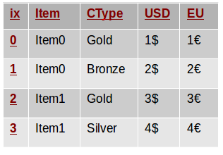
Although the semantics doesn’t matter in this example, you can think of it as a table of items we want to sell. The Item column contains the item names, USD is the price in US dollars and EU is the price in euros. Each client can be classified as Gold, Silver or Bronze customer and this is specified in the CType column.
The following code snippet creates the depicted DataFrame. Note that we will assume these imports are present in all code snippets throughout this article.
1
2
3
4
5
6
7
8
9
10
11
12
from collections import OrderedDict
from pandas import DataFrame
import pandas as pd
import numpy as np

table = OrderedDict((
    ("Item", ['Item0', 'Item0', 'Item1', 'Item1']),
    ('CType',['Gold', 'Bronze', 'Gold', 'Silver']),
    ('USD',  ['1$', '2$', '3$', '4$']),
    ('EU',   ['1€', '2€', '3€', '4€'])
))
d = DataFrame(table)
In such a table, it is not easy to see how the USD price varies over different customer types. We may like to reshape/pivot the table so that all USD prices for an item are on the row to compare more easily. With Pandas, we can do so with a single line:
1
p = d.pivot(index='Item', columns='CType', values='USD')
This invocation creates a new table/DataFrame whose columns are the unique values in d.CType and whose rows are indexed with the unique values of d.Item. So far we have defined the indices of the columns and rows, but what about the cells’ values? This is defined by the last parameter of the invocation - values='USD'. Each cell in the newly created DataFrame will have as a value the entry of the USD column in the original table corresponding to the same Item and CType. The following diagram illustrates this. Column and row indices are marked in red.
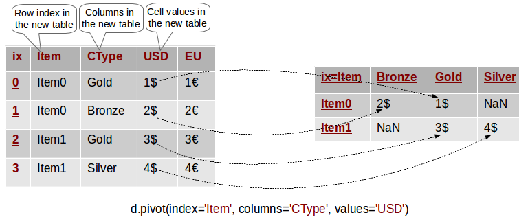
In other words, the value of USD for every row in the original table has been transferred to the new table, where its row and column match the Item and CType of its original row. Cells in the new table which do not have a matching entry in the original one are set with NaN.
As an example the following lines perform equivalent queries on the original and pivoted tables:
1
2
3
4
5
# Original DataFrame: Access the USD cost of Item0 for Gold customers
print (d[(d.Item=='Item0') & (d.CType=='Gold')].USD.values)

# Pivoted DataFrame: Access the USD cost of Item0 for Gold customers
print (p[p.index=='Item0'].Gold.values)
Note that in this example the pivoted table does not contain any information about the EU column! Indeed, we can’t see those euro symbols anywhere! Thus, the pivoted table is a simplified version of the original data and only contains information about the columns we specified as parameters to the pivot method.
Pivoting By Multiple Columns
Now what if we want to extend the previous example to have the EU cost for each item on its row as well? This is actually easy - we just have to omit the values parameter as follows:
1
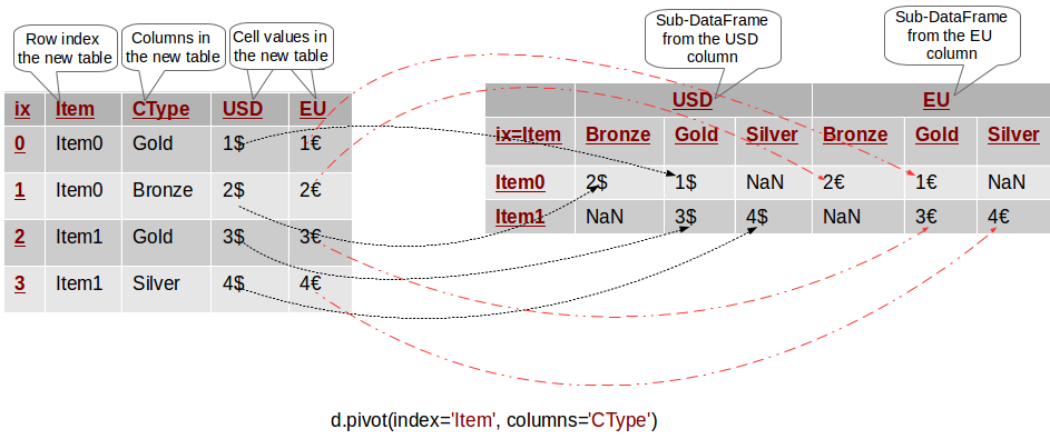
p = d.pivot(index='Item', columns='CType')
In this case, Pandas will create a hierarchical column index (MultiIndex) for the new table. You can think of a hierarchical index as a set of trees of indices. Each indexed column/row is identified by a unique sequence of values defining the “path” from the topmost index to the bottom index. The first level of the column index defines all columns that we have not specified in the pivot invocation - in this case USD and EU. The second level of the index defines the unique value of the corresponding column. This is depicted in the following diagram:
We can use this hierarchical column index to filter the values of a single column from the original table. For example p.USD returns a pivoted DataFrame with the USD values only and it is equivalent to the pivoted DataFrame from the previous section.
To exemplify hierarchical indices, the expression p.USD.Bronze selects the first column in the pivoted table.
As a further example the following queries on the original and pivoted tables are equivalent:
1
2
3
4
5
# Original DataFrame: Access the USD cost of Item0 for Gold customers
print(d[(d.Item=='Item0') & (d.CType=='Gold')].USD.values)

# Pivoted DataFrame: p.USD gives a "sub-DataFrame" with the USD values only
print(p.USD[p.USD.index=='Item0'].Gold.values)
Common Mistake in Pivoting
As we saw the pivot method takes at least 2 column names as parameters - the index and the columns named parameters. What will happen if we have multiple rows with the same values for these columns? How will the pivot method determine the value of the corresponding cell in the pivoted table? The following diagram depicts the problem:
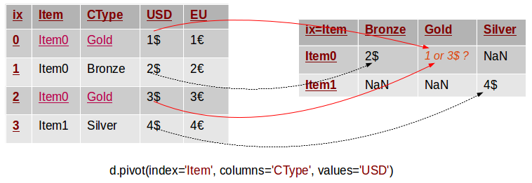
In this example we have two rows with the same values (“Item0” and “Gold”) for the Item and CType columns. The pivot method can not know what should be the value of the corresponding value in the pivoted table. Thus, it throws an exception with the following message:
1
ValueError: Index contains duplicate entries, cannot reshape
The following code reproduces the issue:
1
2
3
4
5
6
7
8
table = OrderedDict((
    ("Item", ['Item0', 'Item0', 'Item0', 'Item1']),
    ('CType',['Gold', 'Bronze', 'Gold', 'Silver']),
    ('USD',  ['1',  '2',  '3',  '4']),
    ('EU',   ['1€', '2€', '3€', '4€'])
))
d = DataFrame(table)
p = d.pivot(index='Item', columns='CType', values='USD')
Hence, before calling pivot we need to ensure that our data does not have rows with duplicate values for the specified columns. If we can’t ensure this we may have to use the pivot_table method instead.
Pivot Table
The pivot_table method comes to solve this problem. It works like pivot, but it aggregates the values from rows with duplicate entries for the specified columns. In other words, in the previous example we could have used the mean, the median or another aggregation function to compute a single value from the conflicting entries. This is depicted in the example below.
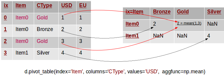
Note that in this example we removed the $ and € symbols to simplify things. There are two rows in the original table, whose values for Item and CType are duplicate. The corresponding value in the pivot table is defined as the mean of these two original values. The pivot_table method takes a parameter called aggfunc, which is the aggregation function used to combine the multitude of values. In this example we used the mean function from numpy. The following snippet lists the code to reproduce the example:
1
2
3
4
5
6
7
8
table = OrderedDict((
    ("Item", ['Item0', 'Item0', 'Item0', 'Item1']),
    ('CType',['Gold', 'Bronze', 'Gold', 'Silver']),
    ('USD',  [1, 2, 3, 4]),
    ('EU',   [1.1, 2.2, 3.3, 4.4])
))
d = DataFrame(table)
p = d.pivot_table(index='Item', columns='CType', values='USD', aggfunc=np.min)
In essence pivot_table is a generalisation of pivot, which allows you to aggregate multiple values with the same destination in the pivoted table.
Stack/Unstack
In fact pivoting a table is a special case of stacking a DataFrame. Let us assume we have a DataFrame with MultiIndices on the rows and columns. Stacking a DataFrame means moving (also rotating or pivoting) the innermost column index to become the innermost row index. The inverse operation is called unstacking. It means moving the innermost row index to become the innermost column index. The following diagram depicts the operations:
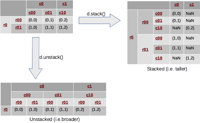
In this example, we look at a DataFrame with 2-level hierarchical indices on both axes. Stacking takes the most-inner column index (i.e. c00, c01, c10), makes it the most inner row index and reshuffles the cell values accordingly. Inversely, unstacking moves the inner row indices (i.e. r00, r01) to the columns.
Typically, stacking makes the DataFrame taller, as it is “stacking” data in fewer columns and more rows. Similarly, unstacking usually makes it shorter and wider or broader. The following reproduces the example:
1
2
3
4
5
6
7
8
9
10
11
12
13
14
15
# Row Multi-Index
row_idx_arr = list(zip(['r0', 'r0'], ['r-00', 'r-01']))
row_idx = pd.MultiIndex.from_tuples(row_idx_arr)

# Column Multi-Index
col_idx_arr = list(zip(['c0', 'c0', 'c1'], ['c-00', 'c-01', 'c-10']))
col_idx = pd.MultiIndex.from_tuples(col_idx_arr)

# Create the DataFrame
d = DataFrame(np.arange(6).reshape(2,3), index=row_idx, columns=col_idx)
d = d.applymap(lambda x: (x // 3, x % 3))

# Stack/Unstack
s = d.stack()
u = d.unstack()
In fact Pandas allows us to stack/unstack on any level of the index so our previous explanation was a bit simplified :). Thus, in the previous example we could have stacked on the outermost index level as well! However, the default (and most typical case) is to stack/unstack on the innermost index level.
Stacking and unstacking can also be applied to data with flat (i.e. non-hierchical) indices. In this case, one of the indices is de facto removed (the columns index if stacking, and the rows if unstacking) and its values are nested in the other index, which is now a MultiIndex. Therefore, the result is always a Series with a hierarchical index. The following example demonstrates this:
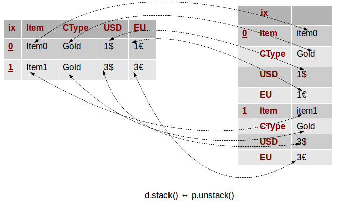
In this example we take a DataFrame similar to the one from the beginning. Instead of pivoting, this time we stack it, and we get a Series with a MultiIndex composed of the initial index as first level, and the table columns as a second. Unstacking can help us get back to our original data structure.